
Diffusion models have emerged as a leading approach in generative modeling, powering advances in image, audio, and text synthesis. This post offers a concise, math-first walkthrough of how they work—from the forward diffusion process to the reverse denoising steps, and the loss functions used during training. Ideal for readers who want to understand the core ideas from the ground up.
Introduction
Diffusion models operate through two key processes: a forward (diffusion) process that corrupts data with noise, and a reverse process that learns to recover the original data.
In the forward process, we take real data (e.g., an image) and gradually add noise to it over several time steps. This process is fixed and does not require learning; it’s usually designed to be a Markov chain, meaning each step only depends on the previous step.
Formally, given a real data sample $\vx_0 \sim q(\vx_0)$, we define a sequence $\vx_1, \dots, \vx_T$, where noise is added at each time step according to a variance schedule $\beta_1, \dots, \beta_T$.
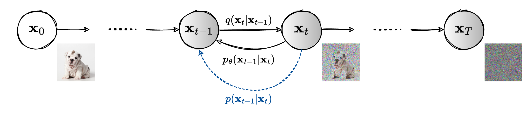 The directed graphical model.
In particular, we have
\[\begin{equation} \label{eq:qxtgivenxtminus1} q(\vx_t\lvert\vx_{t-1}) = \mathcal{N}(\vx_t; \sqrt{1-\beta_t}\vx_{t-1}, \beta_t\id). \end{equation}\]Thanks to the reparameterization we can directly obtain $\vx_t$ from the input $\vx_0$ as
\[\begin{equation} \label{eq:qxtgivenx0} \vx_t = \sqrt{\bar{\alpha}_t} \vx_0 + \sqrt{1 - \bar{\alpha}_t}\boldsymbol{\epsilon}, \end{equation}\]where $\boldsymbol{\epsilon}\sim \mathcal{N}(\vect{0}, \vect{I})$ and $\bar{\alpha}_t$ can be derived in closed form. In particular, by defining $\alpha_t = 1 - \beta_t$, and \(\bar{\alpha}_t = \prod_{i=1}^{t} {\alpha}_i.\)
Proof:
\[\begin{align*} \vx_t &= \sqrt{\alpha_t}\vx_{t-1} + \sqrt{1 - \alpha_t}\boldsymbol{\epsilon}_{t-1} \quad \quad& \boldsymbol{\epsilon}_{t-1} \sim \mathcal{N}(\zeros, \id)\\ &= \sqrt{\alpha_t}(\sqrt{\alpha_{t-1}}\vx_{t-2} + \sqrt{1 - \alpha_{t-1}}\boldsymbol{\epsilon}_{t-2}) + \sqrt{1 - \alpha_t}\boldsymbol{\epsilon}_{t-1}\quad \quad&\boldsymbol{\epsilon}_{t-1}, \boldsymbol{\epsilon}_{t-2} \sim \mathcal{N}(\zeros, \id)\\ &= \sqrt{\alpha_t\alpha_{t-1}}\vx_{t-2} + \sqrt{1 - \alpha_t\alpha_{t-1}}\bar{\boldsymbol{\epsilon}}_{t-2}\quad\quad & (*)\\ &= \dots\\ &= \sqrt{\bar{\alpha}_t}\vx_0 + \sqrt{1 - \bar{\alpha}_t}\boldsymbol{\epsilon} \end{align*}\]$(*)$ Recall that when we merge two Gaussians with different variances, e.g, $\mathcal{N}(\zeros, \sigma_1^2\id)$, $\mathcal{N}(\zeros, \sigma_2^2\id)$, the new distribution is $\mathcal{N}(\zeros, (\sigma_1^2 + \sigma_2^2)\id)$. In this case, the merged standard deviation is \(\sqrt{(1- \alpha_t) + \alpha_t(1 - \alpha_{t-1})} = \sqrt{1 - \alpha_t\alpha_{t-1}}.\)
If we could reverse the process and sample from $q(\vx_{t-1}\lvert\vx_t)$ we could then generate new samples starting from Gaussian noise $\vx_T \sim \mathcal{N}(\vect{0}, \vect{I})$. However, we cannot directly estimate $q(\vx_{t-1}\lvert\vx_t)$, but we can learn $p_{\theta}(\vx_{t-1} \lvert \vx_{t})$.
The joint distribution $p_{\theta}(\vx_{0:T})$ is called the reverse process, and it is defined as a Markov chain with learned Gaussian transitions starting at $p(\vx_{T}) = \mathcal{N}(\vx_{T}; \vect{0}, \vect{I})$.
\[\begin{align*} p_{\theta}(\vx_{0:T}) &\coloneqqf p(\vx_T)\prod_{t=1}^T p_{\theta}(\vx_{t-1}\lvert \vx_t)\\ p_{\theta}(\vx_{t-1}\lvert \vx_t) &\coloneqqf \mathcal{N}(\vx_{t-1}; \boldsymbol{\mu}_{\theta}(\vx_t, t), \boldsymbol{\Sigma}_{\theta}(\vx_t, t)). \end{align*}\]In particular, note that the parameters of the Gaussian distribution depend on the actual step $t$ and not only on the data at that specific step $\vx_t$.
Some math
In order to train the model we need to optimize a certain loss function. Therefore, now we compute some terms which will become useful later.
Reverse conditional probability:
\[\begin{align*} q(\vx_{t-1}\lvert\vx_t, \vx_0) &= q(\vx_{t}\lvert \vx_{t-1}, \vx_0)\frac{q(\vx_{t-1}\lvert \vx_0)}{q(\vx_{t}\lvert \vx_0)} \quad \text{(Bayes'rule)}\\ &\propto \exp\left( - \frac{1}{2} \left(\frac{(\vx_t - \sqrt{\alpha_t}\vx_{t-1})^2}{\beta_t} + \frac{(\vx_{t-1} - \sqrt{\bar{\alpha}_{t-1}}\vx_0)^2}{1 - \bar{\alpha}_{t-1}} - \frac{(\vx_{t} - \sqrt{\bar{\alpha}_{t}}\vx_0)^2}{1 - \bar{\alpha}_{t}} \right) \right) \\ &\text{(applied eq. \eqref{eq:qxtgivenxtminus1} and \eqref{eq:qxtgivenx0})}\\ &= \exp\left( - \frac{1}{2} \left(\frac{\vx_t^2 - 2\sqrt{\alpha_t}\vx_t\textcolor{blue}{\vx_{t-1}} + \alpha_t\textcolor{red}{\vx_{t-1}^2}}{\beta_t} + \frac{\textcolor{red}{\vx_{t-1}^2} - 2\sqrt{\bar{\alpha}_{t-1}}\vx_0\textcolor{blue}{\vx_{t-1}} + \vx_0^2}{1 - \bar{\alpha}_{t-1}} + c(\vx_t, \vx_0) \right) \right)\\ &= \exp \left( - \frac{1}{2} \left( \textcolor{red}{\left(\frac{\alpha_t}{\beta_t} + \frac{1}{1-\bar{\alpha}_{t-1}}\right)\vx_{t-1}^2} - \textcolor{blue}{\left( \frac{2\sqrt{\alpha_t}}{\beta_t}\vx_t + \frac{2\sqrt{\bar{\alpha}_{t-1}}}{1 - \bar{\alpha}_{t-1}}\vx_0 \right) \vx_{t-1}} + c(\vx_t, \vx_0)\right) \right) \end{align*}\]Now we can say that $q(\vx_{t-1}\lvert\vx_t, \vx_0)$ is also Gaussian and that it has a scaled identity covariance with scaling factor equal to $1/\left(\frac{\alpha_t}{\beta_t} + \frac{1}{1-\bar{\alpha}_{t-1}}\right)$ and mean equal to \(\left( \frac{\sqrt{\alpha_t}}{\beta_t}\vx_t + \frac{\sqrt{\bar{\alpha}_{t-1}}}{1 - \bar{\alpha}_{t-1}}\vx_0 \right)/ \left(\frac{\alpha_t}{\beta_t}+ \frac{1}{1-\bar{\alpha}_{t-1}}\right)\).
Notice that the variance is a constant that depends on the step $t$, whereas the mean is a function of both $\vx_t$ and $\vx_0$. However, from eq. \eqref{eq:qxtgivenx0} we can find $\vx_0$ as
\[\begin{equation*} \vx_0 = \textcolor{mybrown}{\frac{1}{\sqrt{\bar{\alpha}_t}} (\vx_t - \sqrt{1 - \bar{\alpha}_t}\boldsymbol{\epsilon})} \end{equation*}\]Because of this, we can write the mean as a function of $\vx_t$ and $\boldsymbol{\epsilon}_t$. However, despite the equation above might suggest something different, always keep in mind the $\vx_t = \vx_t(\vx_0, \boldsymbol{\epsilon})$. With further simplification we can write:
\[\begin{align*} \tilde{\beta}_t &= 1/\left(\frac{\alpha_t}{\beta_t} + \frac{1}{1-\bar{\alpha}_{t-1}}\right)= 1/\left( \frac{\alpha_t - \bar{\alpha}_t + \beta_t}{\beta_t(1- \bar{\alpha}_{t-1})}\right) = \textcolor{ForestGreen}{\frac{1- \bar{\alpha}_{t-1}}{1 - \bar{\alpha}_t}\cdot\beta_t} \end{align*}\]and
Loss function
For the loss function, we consider the variational lower bound on the negative log-likelihood. Remember the expression of the variational lower bound for the variational autoencoder (VAE). There, it was shown that the ELBO is equal to
\[\begin{equation*} \mathcal{L}_{\theta, \phi} = \mathbb{E}_{q_{\phi}(\vz \lvert \vx)}\left[ \log\left[ \frac{p_{\theta}(\vx, \vz)}{q_{\phi}(\vz\lvert\vx)}\right]\right], \end{equation*}\]or, in other words the expectation of the log of the joint distribution of the data and the latent vector, over the inference distribution. Similarly, for the diffusion model we can find an upper bound to the negative log-likelihood. In particular, for diffusion models we do not have a single latent vector as in the VAE, but many, that is $\vx_{1:T}$. Therefore, we can write
\[\begin{equation*} -\log p_{\theta}(\vx_0) \leq - \mathbb{E}_{q(\vx_{1:T}\lvert \vx_0)}\log \left[ \frac{p_{\theta}(\vx_{0:T})}{q(\vx_{1:T}\lvert \vx_0)} \right]. \end{equation*}\]Having this in mind, the next steps are about simplifying the loss function \(\mathbb{E}_{q(\vx_0)} [-\log p_{\theta}(\vx_0)]\). Therefore, let’s start.
Now, let’s simplify the term in the middle $\sum_{t =2}^T \log \frac{q(\vx_t \lvert \vx_{t-1})}{p_{\theta}(\vx_{t-1}\lvert \vx_t)}$. Firstly, we can use the identity
\[\begin{equation*} q(\vx_t \lvert \vx_{t-1}) q(\vx_{t-1}\lvert \vx_0) = q(\vx_{t-1}\lvert \vx_t, \vx_0) q(\vx_t \lvert \vx_0) \end{equation*}\]which implies that
Now, by plugging in Eq. \eqref{eq: useful-eq} we obtain:
\[\begin{align*} \sum_{t =2}^T \log \frac{q(\vx_t \lvert \vx_{t-1})}{p_{\theta}(\vx_{t-1}\lvert \vx_t)} &= \sum_{t =2}^T \log \left( \frac{q(\vx_{t-1}\lvert \vx_t, \vx_0)}{p_{\theta}(\vx_{t-1}\lvert \vx_t)} \cdot \frac{q(\vx_t \lvert \vx_0)}{q(\vx_{t-1}\lvert \vx_0)} \right)\\ &= \sum_{t =2}^T \log \frac{q(\vx_{t-1}\lvert \vx_t, \vx_0)}{p_{\theta}(\vx_{t-1}\lvert \vx_t)} + \sum_{t =2}^T \log \frac{q(\vx_t \lvert \vx_0)}{q(\vx_{t-1}\lvert \vx_0)}\\ &= \sum_{t =2}^T \log \frac{q(\vx_{t-1}\lvert \vx_t, \vx_0)}{p_{\theta}(\vx_{t-1}\lvert \vx_t)} + \log \frac{q(\vx_T \lvert \vx_0)}{q(\vx_{1}\lvert \vx_0)} \\ &\text{(because most of the terms in the fraction simplify)}. \end{align*}\]Now, by plugging in this result into the Eq. \eqref{eq: loss-func-intermediate} we can continue our simplification of the loss.
Now, the question is how to get the expression of the \(\mathbb{E}_q[D_{\mathrm{KL}}(\dots)]\). Let’s remember two important things:
- $D_{\text{KL}}(q \parallel p) = \mathbb{E}_q\left[ \log \frac{q}{p}\right]$
- $\mathbb{E}_q[\dots] = \mathbb{E}_{q(\vx_{0:T})}[\dots]$
Now, let’s focus on the term \(\mathbb{E}_q\left[ \log \frac{q(\vx_{\tau-1}\lvert \vx_{\tau}, \vx_0)}{p_{\theta}(\vx_{\tau-1}\lvert \vx_{\tau})}\right]\) for a generic $\tau > 1$, which appears in the second term of the loss function inside the sum. Therefore, we obtain
\[\begin{align*} \mathbb{E}_q\left[ \log \frac{q(\vx_{\tau-1}\lvert \vx_{\tau}, \vx_0)}{p_{\theta}(\vx_{\tau-1}\lvert \vx_{\tau})}\right] &= \mathbb{E}_{q(\vx_0)q(\vx_T \lvert \vx_0)\prod_{t>1, t\neq\tau}^T q(\vx_{t-1}\lvert \vx_t, \vx_0)} \left[ \mathbb{E}_{q(\vx_{\tau -1}\lvert \vx_{\tau}, \vx_0)} \left[ \log \frac{q(\vx_{\tau-1}\lvert \vx_{\tau}, \vx_0)}{p_{\theta}(\vx_{\tau-1}\lvert \vx_{\tau})}\right] \right]\\ &= \mathbb{E}_{q(\vx_0)q(\vx_T \lvert \vx_0)\prod_{t>1, \textcolor{blue}{t\neq\tau}}^T q(\vx_{t-1}\lvert \vx_t, \vx_0)} \left[ D_{\text{KL}}(q(\vx_{\tau-1}\lvert \vx_{\tau}, \vx_0)\parallel p_{\theta}(\vx_{\tau-1}\lvert \vx_{\tau})) \right]\\ &= \mathbb{E}_{q(\vx_0)q(\vx_T \lvert \vx_0)\prod_{t>1}^T q(\vx_{t-1}\lvert \vx_t, \vx_0)} \left[ D_{\text{KL}}(q(\vx_{\tau-1}\lvert \vx_{\tau}, \vx_0)\parallel p_{\theta}(\vx_{\tau-1}\lvert \vx_{\tau})) \right] \quad \textcolor{blue}{(**)}\\ &= \mathbb{E}_{q} \left[ D_{\text{KL}}(q(\vx_{\tau-1}\lvert \vx_{\tau}, \vx_0)\parallel p_{\theta}(\vx_{\tau-1}\lvert \vx_{\tau}))\right] \end{align*}\]$\textcolor{blue}{(**)}$ Since the KL term involves taking an expectation over $\vx_{\tau - 1}$ it results in a term that is constant with respect to $\vx_{\tau - 1}$ so if you take the expectation over it again with respect to a distribution over $\vx_{\tau - 1}$ it is left unchanged. Regarding \(\mathbb{E}_q\left[ \log \frac{q(\vx_T \lvert \vx_0)}{p_{\theta}(\vx_T)} \right]\) we can repeat the same reasoning.
Therefore, the final loss function reads as
Every KL term (except for $L_0$) compares two Gaussian distributions, therefore can be computed in closed form. $L_T$ is constant and can be ignored during training because $q$ has no learnable parameters and $\vx_T$ is a Gaussian noise. Ho et al. 2020 models $L_0$ using a separate discrete decoder derived from $\mathcal{N}(\vx_0;\boldsymbol{\mu}_{\theta}(\vx_1, 1), \boldsymbol{\Sigma}_{\theta}(\vx_1, 1))$.
Parametrization of $L_{t-1}$
Recall that the KL Divergence between two Gaussian distributions is:
\[\begin{equation*} D_{\text{KL}}(\mathcal{N}(\vx; \boldsymbol{\mu}_x, \boldsymbol{\Sigma}_x) \parallel \mathcal{N}(\vy; \boldsymbol{\mu}_y, \boldsymbol{\Sigma}_y)) = \frac{1}{2}\left[ \log \frac{\abs{\boldsymbol{\Sigma}_y}}{\abs{\boldsymbol{\Sigma}_x}} -d + \trace(\boldsymbol{\Sigma}_y^{-1}\boldsymbol{\Sigma}_x) + (\boldsymbol{\mu}_y - \boldsymbol{\mu}_x)^{\Tr}\boldsymbol{\Sigma_y}^{-1} (\boldsymbol{\mu}_y - \boldsymbol{\mu}_x) \right] \end{equation*}\]In our case the two distributions with respect to which we have to compute the KL Divergence are:
- $q(\vx_{t-1}\lvert \vx_t, \vx_0) = \mathcal{N}(\vx_{t-1}; \tilde{\boldsymbol{\mu}}_t, \tilde{\beta}_t\id)$
- $p_{\theta}(\vx_{t-1}\lvert \vx_t) = \mathcal{N}(\vx_{t-1}; \boldsymbol{\mu}_{\theta}(\vx_t, t), \boldsymbol{\Sigma}_{\theta}(\vx_t, t)) = \mathcal{N}(\vx_{t-1}; \boldsymbol{\mu}_{\theta}(\vx_t, t), \sigma_t^2\id)$.
Therefore, we obtain
By plugging in the result of $\tilde{\boldsymbol{\mu}}_t$ we obtain
When looking at Eq. \eqref{eq: loss-diff-means} we can see that in order to predict $\boldsymbol{\mu}_{\theta}(\vx_t(\vx_0, \boldsymbol{\epsilon}), t)$ we have to
- sample $\vx_0 \sim q(\vx_0)$, $\boldsymbol{\epsilon} \sim \mathcal{N}(\zeros, \id)$
- find $\vx_t$ with Eq. \eqref{eq:qxtgivenx0}
- predict $\boldsymbol{\mu}_{\theta}(\vx_t(\vx_0, \boldsymbol{\epsilon}), t)$
However, since $\boldsymbol{\mu}_{\theta}(\vx_t(\vx_0, \boldsymbol{\epsilon}), t)$ must predict $\tilde{\boldsymbol{\mu}}_t = \frac{1}{\sqrt{\alpha_t}}(\vx_t(\vx_0, \boldsymbol{\epsilon}) - \frac{1-\alpha_t}{\sqrt{1 - \bar{\alpha}_t}}\boldsymbol{\epsilon})$, we can choose a similar form for the mean. That is
In this way, the procedure described above changes as:
- sample $\vx_0 \sim q(\vx_0)$, $\boldsymbol{\epsilon} \sim \mathcal{N}(\zeros, \id)$
- find $\vx_t$ with Eq. \eqref{eq:qxtgivenx0}
- predict $\boldsymbol{\epsilon}_{\theta}(\vx_t, t)$
- estimate $\boldsymbol{\mu}_{\theta}(\vx_t(\vx_0, \boldsymbol{\epsilon}), t)$ with Eq. \eqref{eq: mean-wrt-epsilon}
With this reparametrization Eq. \eqref{eq: loss-diff-means} simplifies as
This means that by optimizing this loss we try to predict the realization of the noise $\boldsymbol{\epsilon} \sim \mathcal{N}(\zeros, \id)$ that determines $\vx_t$ from $\vx_0$. Without the weighting factor all the terms, including $L_0$, converge to the expression \(\norm{\boldsymbol{\epsilon}_{\theta}(\vx_t, t) - \boldsymbol{\epsilon}}\). Additionally, by scaling all the term by the factor $\frac{1}{T}$ we can convert the $\sum_{t=1}^T$ into the expectation over $t\sim \mathcal{U}[1, T]$. This explains the training procedure described in (Ho et al., 2020).
The references which have been used so far are (Ho et al., 2020; Luo, 2022; Weng, 2021)
Equivalent Interpretations of the Loss Function
Let’s go back to the original loss function in Eq. \eqref{eq: loss-diff-means-prelim} where we obtained
\[\begin{equation*} L_{t-1} - const. = \mathbb{E}_q\left[ \frac{1}{2\sigma_t^2}\norm{\boldsymbol{\mu}_{\theta}(\vx_t, t) - \tilde{\boldsymbol{\mu}}_t}^2\right] \end{equation*}\]Before, in order the reach the desired expression for the loss function we have written $\tilde{\boldsymbol{\mu}}_t$ as function of $\vx_t$ and $\boldsymbol{\epsilon}$. In the following we will present two other different options of expressing the mean which will lead to other two different expressions of the final loss function.
Option 1
The first option consists in keeping the former expression of $\tilde{\boldsymbol{\mu}}_t$ as a function of $\vx_t$ and $\vx_0$.
Based on this expression we can now set $\boldsymbol{\mu}_{\theta}(\vx_t, t)$ to exactly match this expression as
With this in mind we can rewrite the loss function as:
which means that the goal becomes learning a neural network that predicts the original ground truth image from an arbitrarily noisified version of it. Note that the expectation is with respect to both $\vx_0$ and $\boldsymbol{\epsilon}$, because $\vx_t$ is a function of these two random variables.
Option 2
To derive the third interpretation of the loss function we can use Tweedie’s Formula (Efron, 2011), which states that the true mean of an exponential family distribution can be estimated by the maximum likelihood of the samples plus some correction term involving the score of the estimate. For a Gaussian random variable $\vz \sim \mathcal{N}(\boldsymbol{\mu}_z, \boldsymbol{\Sigma}_z)$, Tweedie’s formula states that:
Formula \eqref{eq:qxtgivenx0} shows that
\[\begin{equation*} q(\vx_t\lvert \vx_0) = \mathcal{N}(\sqrt{\bar{\alpha}_t}\vx_0, (1- \bar{\alpha}_t)\id). \end{equation*}\]Hence, we can apply Tweedie’s formula also in this case to obtain
\[\begin{equation*} \mathbb{E}[\boldsymbol{\mu}_{x_t}\lvert \vx_t] = \vx_t + (1 - \bar{\alpha}_t)\nabla_{\vx_t}\log p(\vx_t). \end{equation*}\]By utilizing the fact that the mean $\boldsymbol{\mu}_{x_t}$ must be equal to $\sqrt{\bar{\alpha}_t}\vx_0$ we obtain:
Now, we can substitute the value that we obtained for $\vx_0$ in the former expression of $\tilde{\boldsymbol{\mu}}_t$ which is also reported in Eq. \eqref{eq: option-1}. By plugging in the result in Eq. \eqref{eq: x0wrtnabla} we obtain:
Therefore, we can also use this parametrization for the mean:
Then, the corresponding loss function becomes
Therefore, in this case $\vs_{\theta}(\vx_t, t)$ is a neural network that tries to predict the score function $\nabla_{\vx_t}\log p(\vx_t)$, which is the gradient of $\vx_t$ in the data space, for any arbitrary noise level $t$.
As additional comment, in (Luo, 2022) (at page 17) it has been shown that by comparing the two expressions derived for $\vx_0$, namely the one that depends on $\boldsymbol{\epsilon}$ and the one that depends on the score $\nabla_{\vx_t}\log p(\vx_t)$, one can show that to move in the data space in order to maximize the log probability is equivalent to modeling the negative of the source noise (up to a scaling factor).
References
- Ho, J., Jain, A., & Abbeel, P. (2020). Denoising Diffusion Probabilistic Models. Advances in Neural Information Processing Systems, 2020-Decem(NeurIPS 2020), 1–25.
- Luo, C. (2022). Understanding Diffusion Models: A Unified Perspective. 1–23. http://arxiv.org/abs/2208.11970
- Weng, L. (2021). What are diffusion models? Lilianweng.github.io. https://lilianweng.github.io/posts/2021-07-11-diffusion-models/
- Efron, B. (2011). Tweedie’s Formula and Selection Bias. Journal of the American Statistical Association, 106(496), 1602–1614. https://doi.org/10.1198/jasa.2011.tm11181