Maximum Mean Discrepancy

During the second year of my PhD, when I was in need of inspiration, I stumbled upon a remarkable metric that changed everything: the Maximum Mean Discrepancy (MMD). Since the MMD turned things around for me, I want to share why this metric is so powerful and how you can use it to build a two-sample test.

$ \newcommand{\vect}[1]{\boldsymbol{#1}} \newcommand{\vx}{\vect{x}} \newcommand{\vy}{\vect{y}} \newcommand{\va}{\vect{a}} \newcommand{\vb}{\vect{b}} \DeclareMathOperator{\mmd}{MMD} \newcommand{\coloneqqf}{\mathrel{\vcenter{:}}=} \newcommand{\norm}[1]{\left\lVert #1 \right\rVert} \binoppenalty=10000 \relpenalty=10000 $

Let $\vx$ and $\vy$ be random variables defined over a topological space $\mathcal{X}$. Given the observations $X \coloneqqf { \vx_1, \dots, \vx_m }$ and $Y \coloneqqf { \vy_1, \dots, \vy_n}$, i.i.d. from $\mathbb{P}$ and $\mathbb{Q}$, respectively, and we aim to determine whether $\mathbb{P} \neq \mathbb{Q}$.

Definition:

$$\begin{equation} \label{eq:mmd_def} \mmd(\mathbb{P}, \mathbb{Q}, \mathcal{F}) \coloneqqf \sup_{f \in \mathcal{F}}(\mathbb{E}_{\vx \sim \mathbb{P}}[f(\vx)] - \mathbb{E}_{\vy \sim \mathbb{Q}}[f(\vy)]). \end{equation}$$

where $\mathcal{F}$ is a class of functions such that $f:\mathcal{X}\rightarrow \mathbb{R}$.

A biased estimate of the MMD can be obtained by replacing the expectations in \eqref{eq:mmd_def} with the empirical means computed with the samples $X$ and $Y$.

$$\begin{equation} \label{eq:mmd_biased} \widehat{\mmd}_b(X, Y, \mathcal{F}) \coloneqqf \sup_{f \in \mathcal{F}}\left(\frac{1}{m}\sum_{i=1}^m f(\vx_i) - \frac{1}{n}\sum_{j=1}^n f(\vy_j)\right). \end{equation}$$

In particular, to have that the MMD is a valid distance metric, we must identify a class of functions $\mathcal{F}$ that guarantees that $\mmd(\mathbb{P}, \mathbb{Q}, \mathcal{F}) = 0$ if and only if $\mathbb{P} = \mathbb{Q}$. A possible solution is to choose $\mathcal{F}$ to be the unit ball in a reproducing kernel Hilbert space (RKHS).

MMD in RKHS

A RKHS is a Hilbert space of functions generated by a kernel $k$. As the RKHS uniquely determines $k$, we can get rid of the supremum in \eqref{eq:mmd_def} and we can write the expression for the $\mmd^2$ as

$$ \begin{equation} \mmd^2(\mathbb{P}, \mathbb{Q}, \mathcal{F}) = \mathbb{E}_{\vx,\vx' \sim \mathbb{P}} [k(\vx, \vx')] + \mathbb{E}_{\vy,\vy' \sim \mathbb{Q}} [k(\vy, \vy')] - 2\mathbb{E}_{\vx\sim \mathbb{P} ,\vy \sim \mathbb{Q}}[k(\vx, \vy)], \end{equation} $$

Given the samples $\{ \vx_{i} \}^m_{i=1} \stackrel{\text{iid}}{\sim}\mathbb{P}$ and $\{ \vy_{j} \}^n_{j=1} \stackrel{\text{iid}}{\sim}\mathbb{Q}$, and with the help of U-statistics an unbiased empirical estimator can be obtained as

$$\begin{equation} \label{eq:mmd-emp} \widehat{\mmd}^2(X, Y, \mathcal{F}) = \frac{1}{m(m-1)}\sum_{i=1}^m\sum_{j\neq i}^m k(\vx_i, \vx_j) + \frac{1}{n(n-1)}\sum_{i=1}^n\sum_{j\neq i}^n k(\vy_i, \vy_j) - \frac{2}{mn}\sum_{i=1}^m\sum_{j=1}^n k(\vx_i, \vy_j). \end{equation}$$

This result is particularly interesting as it shows that the MMD estimator can be directly computed using a kernel $k$ and a finite set of samples and does not require any density estimation contrarily to what happens when using, e.g., KL divergence.

Two Sample Test

Coming back to our original goal, we are going to use the MMD in the framework of statistical hypothesis testing. For simplicity, we assume that the number of samples for the two distributions is equal ($m=n$).

In particular, the statistical test $T$, is used to distinguish between the null hypothesis $H_0\colon \mathbb{P} = \mathbb{Q}$ and the alternative hypothesis $H_1\colon \mathbb{P} \neq \mathbb{Q}$. Knowing that the MMD is equal to zero if and only if the two distributions are the same, we can compare the $\widehat{\mmd}^2(X, Y, \mathcal{F})$ with a critical value or a threshold: if the threshold is exceeded, then the test rejects the null hypothesis. However, in a finite-sample setting two types of errors can occur: a Type I error, i.e., the error of rejecting the null hypothesis despite the null hypothesis being true, and a Type II error, i.e., the error of accepting the null hypothesis despite $\mathbb{P} \neq \mathbb{Q}$.

A common choice for the threshold is the $(1-\alpha)\text{-quantile}$ of the distribution of the statistic assuming $H_0$ true. The quantity $\alpha$, called the level of the test, must be chosen in advance and ensures that the Type I error does not exceed $\alpha$, i.e., $\Pr(\text{reject }H_0\lvert H_0 \text{ true}) \leq \alpha$. Additionally, when a sufficiently large number of samples is available the Type II error is zero.

In (Gretton et al., 2012), it has been shown that when $\mathbb{P} = \mathbb{Q}$, $\widehat{\mmd}^2(X, Y, \mathcal{F})$ follows an infinite weighted sum of chi-squares as $m\rightarrow \infty$, whereas when $\mathbb{P} \neq \mathbb{Q}$, the statistic is asymptotically normal distributed with the mean equal to $\mmd^2(\mathbb{P}, \mathbb{Q}, \mathcal{F})$ and a variance in the order of $\mathcal{O}(m^{-1})$.

In Figure 1, below we illustrate the distribution of $\widehat{\mmd}^2$ under the two hypotheses.

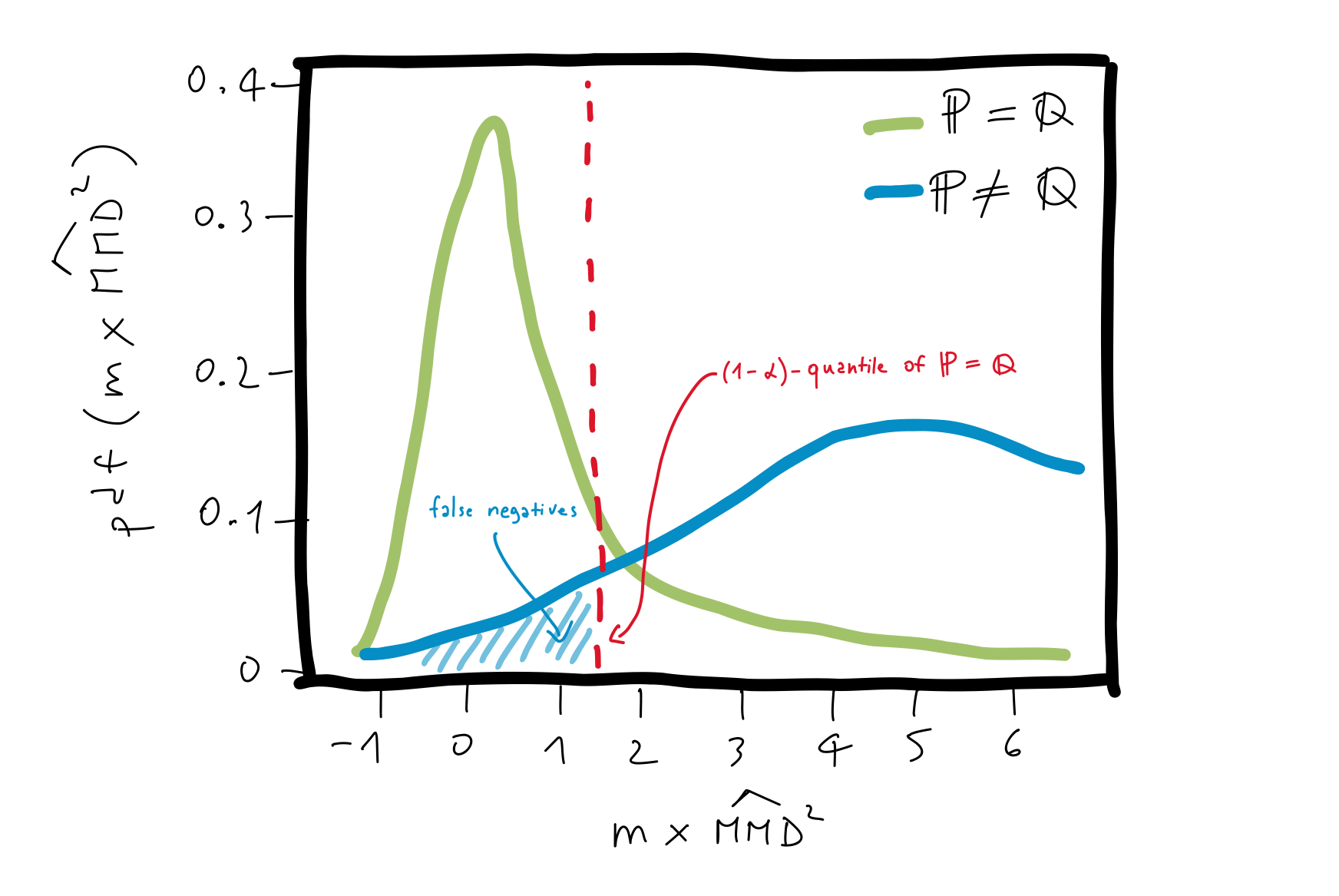Figure 1: Asymptotics of $\widehat{\mmd}^2$.

To have an intuition about this procedure consider the following example.

Example

In this example, we consider a set $X$ of $100$ samples of the digit “$0$” and a set $Y$ of $100$ samples of the digit “$1$”, extracted from the handwritten digits’ dataset (Alpaydin & Kaynak, 1998).

In Figure 2 we observe the heat-map of the values of the kernel between all the combinations of pairs of samples. For the computation, we have chosen a simple Gaussian kernel, that is:

$$\begin{equation} k_{\sigma}(\va, \vb) = \exp\left(-\frac{1}{\sigma^2} \norm{\va - \vb}^2\right), \end{equation}$$

with $\sigma$ chosen accordingly to the median heuristic (Gretton et al., 2012).

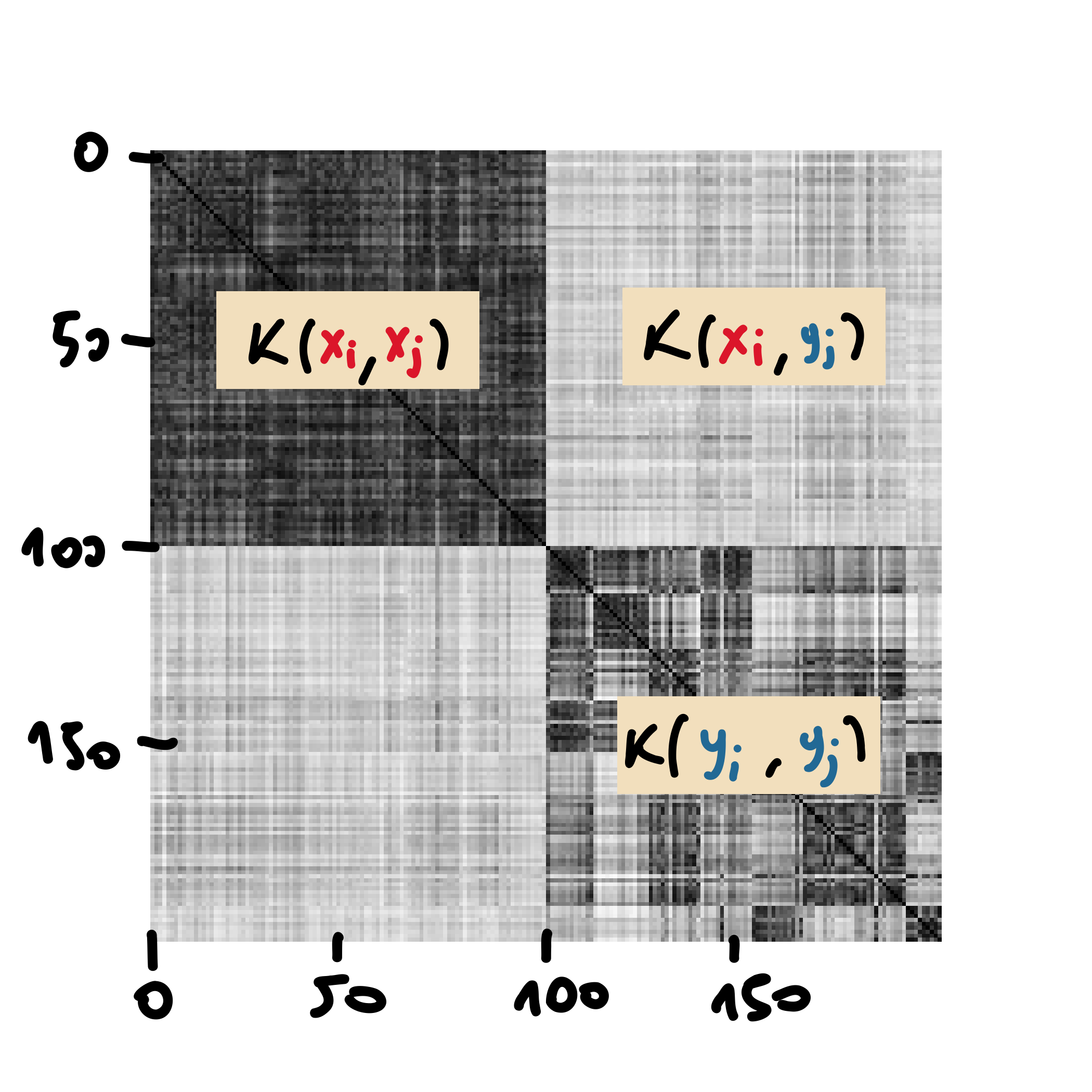Figure 2: Heat-map of the kernels between the samples $X$ and $Y$.

Since in this case $\mathbb{P} \neq \mathbb{Q}$, when evaluating \eqref{eq:mmd-emp} we obtain a relative large value for the resulting $\widehat{\mmd}^2$. This can be observed in Figure 2, where the values on the top-right and bottom-left¹, which correspond to the light areas, are subtracted from the sum of the values on the top-left and bottom-right, which correspond to the dark areas.

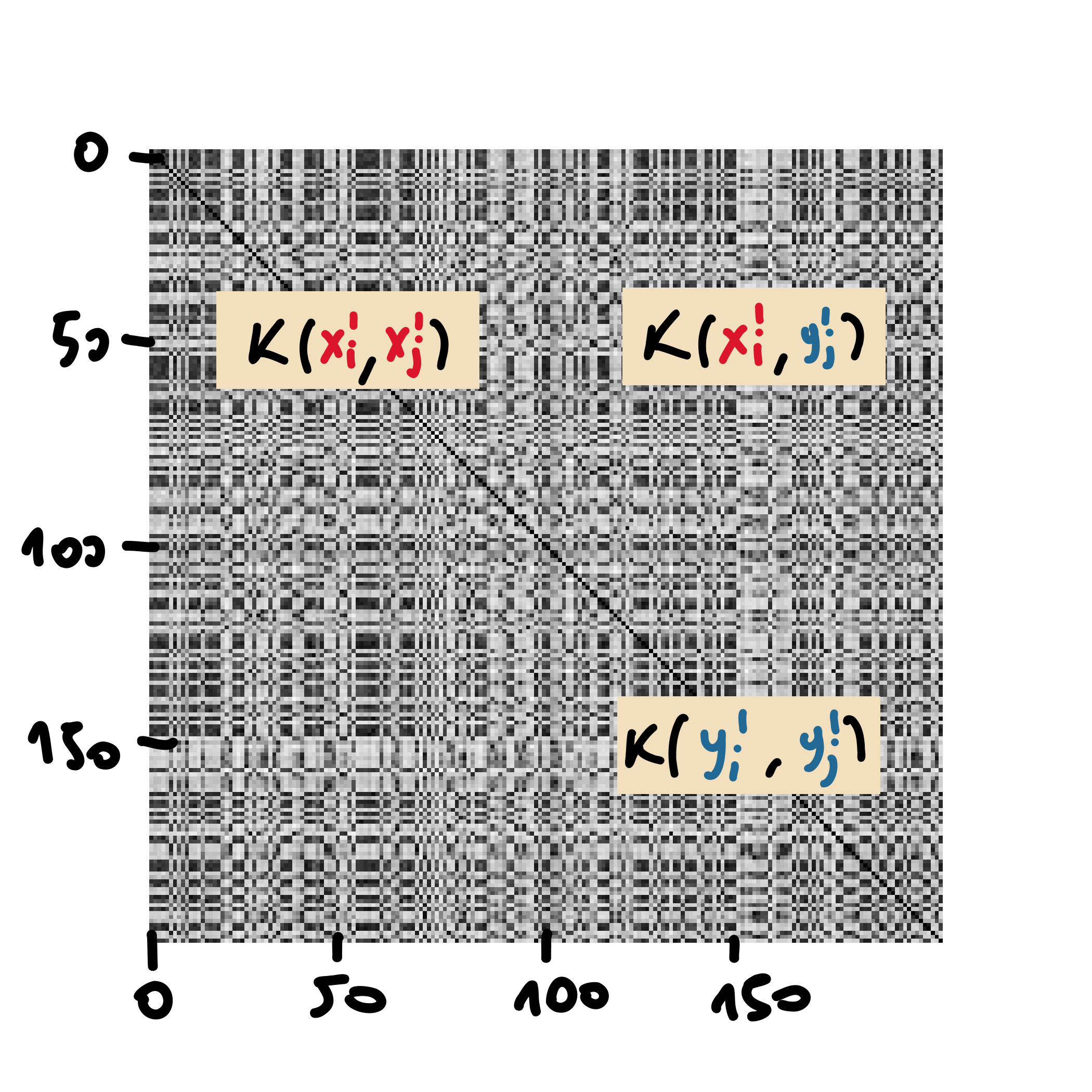Figure 3: Heat-map of the kernels between the samples $X’$ and $Y’$, obtained by randomly partitioning the samples $X \cup Y$.

Now, we have everything that we need to construct the test, given a finite number of samples $m$ from the two distributions $\mathbb{P}$ and $\mathbb{Q}$. For clarity, the Algorithm below shows the pseudocode for the two-sample test considering $N_{\text{perm}} \in \mathbb{N}$ permutations, and given $X$,$Y$, and $\alpha$ as inputs.

Algorithm Two-sample test
$\quad$Inputs: step size $X$, $Y$, $\alpha$, $(\alpha$ is typically small ($\alpha=0.05$))
$\quad \tau \gets \widehat{\mmd}^2(X, Y, k)$
$\quad p_v\gets 0$ (simulate $p$-value via permutations)
$\quad $For $i=1$ to $N_{\text{perm}}$:
$\qquad$Randomly partition $X \cup Y$ into $X’$ and $Y’$
$\qquad$If $\widehat{\mmd}^2(X’, Y’, k) > \tau$:
$\qquad\quad p_v \gets p_v + 1/ N_{\text{perm}}$
$\quad$ If $p_v < \alpha$:
$\qquad$ Return 1 (reject $H_0$)
$\quad$ Else:
$\qquad$ Return 0 (accept $H_0$)

The astute reader might have already noticed that the choice of the kernel has a high impact on the effectiveness of the test. As pointed out in (Gretton et al., 2012), the Gaussian kernel with $\sigma$ chosen to be the median distance between points in the aggregate sample represents a valid choice. However, the design of the optimal kernel, the one that maximizes $\Pr(\text{reject }H_0\lvert H_1\text{ true})$ ², is an ongoing area of research. The study in (Ramdas et al., 2015) has revealed that the power of the kernel based two-sample tests decays with high dimensional data. The recent advances in the area have shown that learning kernels with deep neural networks improve the power of the test (Liu et al., 2020).

Wishing you all a very merry Christmas!

HoHoHo.

References

1. Gretton, A., Borgwardt, K. M., Rasch, M. J., Schölkopf, B., & Smola, A. (2012). A Kernel Two-Sample Test. J. Mach. Learn. Res., 13, 723–773.
2. Alpaydin, E., & Kaynak, C. (1998). Optical Recognition of Handwritten Digits. UCI Machine Learning Repository.
3. Ramdas, A., Reddi, S. J., Póczos, B., Singh, A., & Wasserman, L. (2015). On the Decreasing Power of Kernel and Distance Based Nonparametric Hypothesis Tests in High Dimensions. Proc. AAAI Conf. Artif. Intell.
4. Liu, F., Xu, W., Lu, J., Zhang, G., Gretton, A., & Sutherland, D. J. (2020). Learning Deep Kernels for Non-Parametric Two-Sample Tests. Proc. Int. Conf. Mach. Learn.

1. The values on the top-right and bottom-left are the same because the kernel is symmetric. ↩

2. This quantity is the so-called test power. ↩