Neural Compression

Data compression has always been an important aspect in research. Codecs are tools that compress and decompress digital media, such as image, video, or audio data. Recently, neural codecs have become state-of-the-art, as they often outperform traditional codecs in quality-per-bit, especially at low bitrates. In this post we focus on image compression, and we explore the factorized prior model proposed by Ballé et al. in the paper “Variational image compression with a scale hyperprior”.

Model

The model is composed of the following main components:

• Encoder $g_{\text{a}}$: A neural network that transforms the input image $\boldsymbol{x} \in \mathbb{R}^{3 \times W \times H}$ into a latent representation $\boldsymbol{y} \in \mathbb{R}^{M \times w \times h}$.

• Quantization: A process that converts the latent representation $\boldsymbol{y}$ into a discrete set of values $\hat{\boldsymbol{y}}$.

• Entropy Coding: A method that losslessly compresses the quantized representation. This produces a bit stream from which the quantized representation $\hat{\boldsymbol{y}}$ can be perfectly reconstructed during decoding.

• Decoder $g_{\text{s}}$: A neural network that maps the reconstructed latent representation $\hat{\boldsymbol{y}}$ back into the reconstructed image $\hat{\boldsymbol{x}}$.

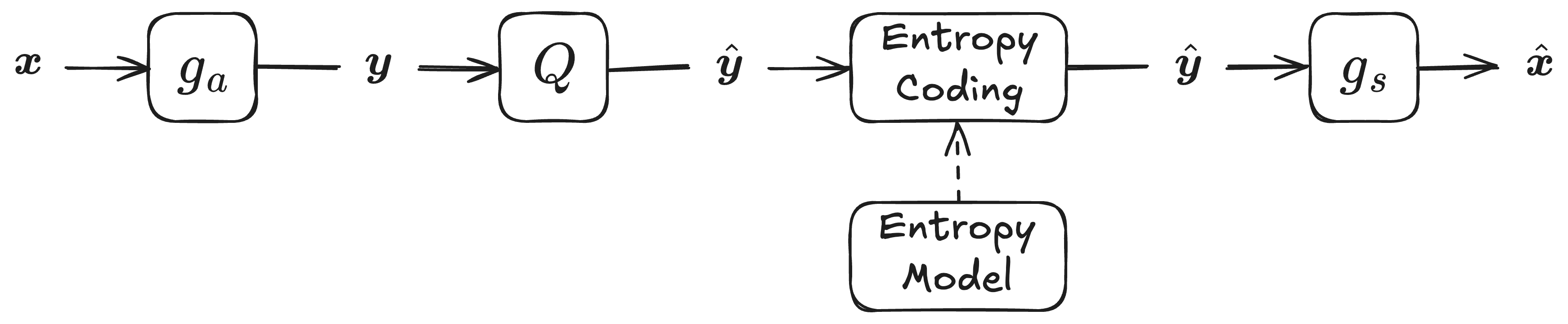Compression schema.

Quantization

During inference the quantization for each element of $\boldsymbol{y}$ is computed as:

\[\begin{equation} \hat{y}_{c, i, j} = \text{round}\left( y_{c, i, j}\right), \end{equation}\]

where $\text{round}(\cdot)$ is the operation of rounding a value to the nearest integer.

However, the $\text{round}(\cdot)$ function it is not differentiable. As a result, it is not used directly during training. Instead, the effect of quantization is approximated by adding uniform noise in the range $[-\frac{1}{2}, \frac{1}{2}]$.

To understand why this is a good solution, let’s consider the quantization noise $\epsilon$.

$\epsilon$ is defined as: \(\begin{equation} y_{c, i, j} - \hat{y}_{c, i, j} = y_{c, i, j} - \text{round}(y_{c, i, j}), \end{equation}\) and lies in the interval $[-\frac{1}{2}, \frac{1}{2}]$ for any $y_{c, i, j} \in \mathbb{R}$.

By assuming that $y_{c, i, j}$ is a uniformly distributed random variable with zero mean that spans a sufficiently large (ideally unbounded) range, we can model the quantization noise as: \(\begin{equation} \epsilon \sim \text{Uniform}\left[-\frac{1}{2}, \frac{1}{2}\right]. \end{equation}\)

Therefore, the model used during training is the one shown in the figure below.

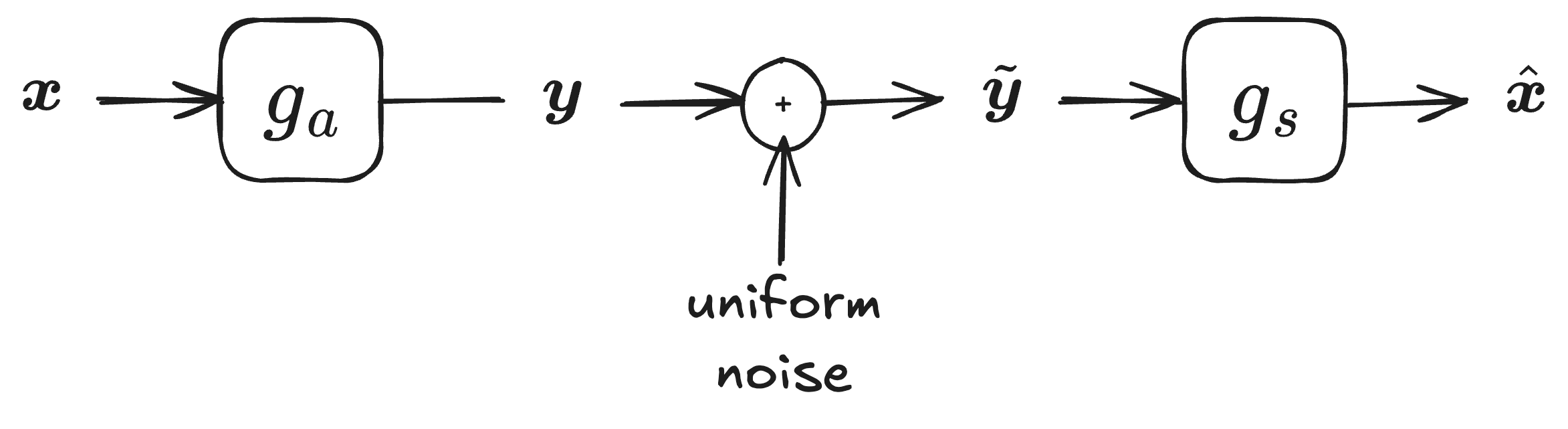Training model.

Entropy coding

Entropy coding can be summarized in three steps:

1. A prior model estimates the probability distribution $p(z)$ for each possible symbol $z \in \mathbb{Z}$.
2. The quantized latent representation $\hat{y}_{c, i, j}$ is entropy encoded using this predicted distribution. Symbols with higher probability are assigned shorter codes, while less probable symbols receive longer codes. The ideal code length for a symbol is $-\log_2 p(z)$ bits (Note that, real-world encoders (like Huffman or arithmetic/range coding) can only approximate this bound).
3. During decoding, the same prior model is used to reconstruct the probability distribution, allowing the bit stream to be decoded losslessly.

Ballé et al. (Ballé et al., 2018) consider a factorized prior over the latent representation. Specifically, they assume that all elements in the $c$-th channel of the quantized latent variable $\hat{\boldsymbol{y}}$ are independent and identically distributed (i.i.d.). Therefore,

\[\begin{equation} p_{\hat{y}_{c, i, j}}=p_{\hat{y}_{c}}. \end{equation}\]

For entropy estimation, the discrete probability mass function (PMF) of $\hat{y}_{c, i, j}$ is approximated using the corresponding cumulative distribution function (CDF) $F_c$:

$$\begin{equation} p_{\hat{y}_{c}}(\hat{y}_{c, i, j}) = F_{c}(\hat{y}_{c, i, j} + 1/2) − F_{c}(\hat{y}_{c, i, j} − 1/2), \end{equation}$$

where $F_c$ is modelled using a small fully-connected neural network (see Section 6.1 of (Ballé et al., 2018) for more details).

Note that, the entropy model is trained separately during training. This will become clear in the next section.

The total number of bits needed to encode $\hat{\boldsymbol{y}}$ is

$$\begin{equation} R_{\hat{\boldsymbol{y}}} = -\log_2 p_{\hat{\boldsymbol{y}}}(\hat{\boldsymbol{y}}) = \sum_{c, i, j} - \log_2 p_{\hat{y}_c} (\hat{y}_{c, i, j}) . \end{equation}$$

Loss function

We aim to optimize two competing objectives: minimizing the length of the bit stream and minimizing distortion, e.g. the mean squared error (MSE) between the original image $\boldsymbol{x}$ and its reconstruction $\hat{\boldsymbol{x}}$.

Accordingly, the loss function is defined as:

$$ \begin{equation} \mathcal{L} = \mathbb{E}_{\boldsymbol{x}} \left[ -\log_2 p_{\tilde{\boldsymbol{y}}}(\tilde{\boldsymbol{y}}) + \lambda \| \boldsymbol{x} - \hat{\boldsymbol{x}} \|_2^2 \right], \end{equation} $$

where $\lambda > 0$ is a hyperparameter that controls the trade-off between rate and distortion. Note that we use the noisy latent representation $\tilde{\boldsymbol{y}}$ in place of the quantized version $\hat{\boldsymbol{y}}$ during training to enable backpropagation through the rate term (see previous discussion).

References

1. Ballé, J., Minnen, D., Singh, S., Hwang, S. J., & Johnston, N. (2018). Variational image compression with a scale hyperprior. International Conference on Learning Representations.