Neural Operators Basics

Neural operators are emerging as a powerful framework for solving partial differential equations using deep learning. This story covers the basics of neural operators. We show how to derive a neural operator layer starting from a simple fully connected layer. Then we also derive the Fourier neural operator, and we show some results on the Darcy flow dataset.

Introduction

Neural operators enable machine learning directly on function spaces. Unlike traditional neural networks, which operate on fixed-dimensional inputs like $64\times64$ images, neural operators are designed to handle inputs and outputs that are functions—potentially defined over continuous domains or discretized at varying resolutions. This means the same model can generalize across different discretizations of the input and output spaces, making it resolution-invariant and particularly well-suited for problems in scientific computing and PDE modeling.

From Neural Networks to Neural Operators

Let’s consider a fully connected layer of a neural network:

\[\begin{equation} v_i = \sigma \left( \sum_{j}^n K_{ij} a_j \right) \end{equation}\]

where $\boldsymbol{a}$ is our input vector and $\boldsymbol{K}$ is a weight matrix and $\sigma$ is a non-linearity.

Now we can interpret the input as a function sampled at points $x_j$, and then we can also assume that $v$ is a function that can be evaluated at any query point $y_i$. Next, instead of thinking to $K_{ij}$ as abstract entries, we can think of them as depending on the location:

\[\begin{equation} K_{ij} = \kappa(y_i, x_j) . \end{equation}\]

Therefore, we can rewrite the equation as:

\[\begin{equation} v(y_i) = \sigma \left( \sum_{j}^n \kappa(y_i, x_j) a(x_j) \Delta x_j \right), \end{equation}\]

where we replaced $1/n$ with $\Delta x_j$.

Then if we replace the sum with the integral we get:

\[\begin{equation} \label{eq:basic-def} v(y_i) = \sigma \left( \int \kappa(y_i, x_j) a(x_j) \text{d}x \right). \end{equation}\]

The figure below illustrates the parallelism between a linear layer and a linear integral operator, highlighting all the steps previously discussed.

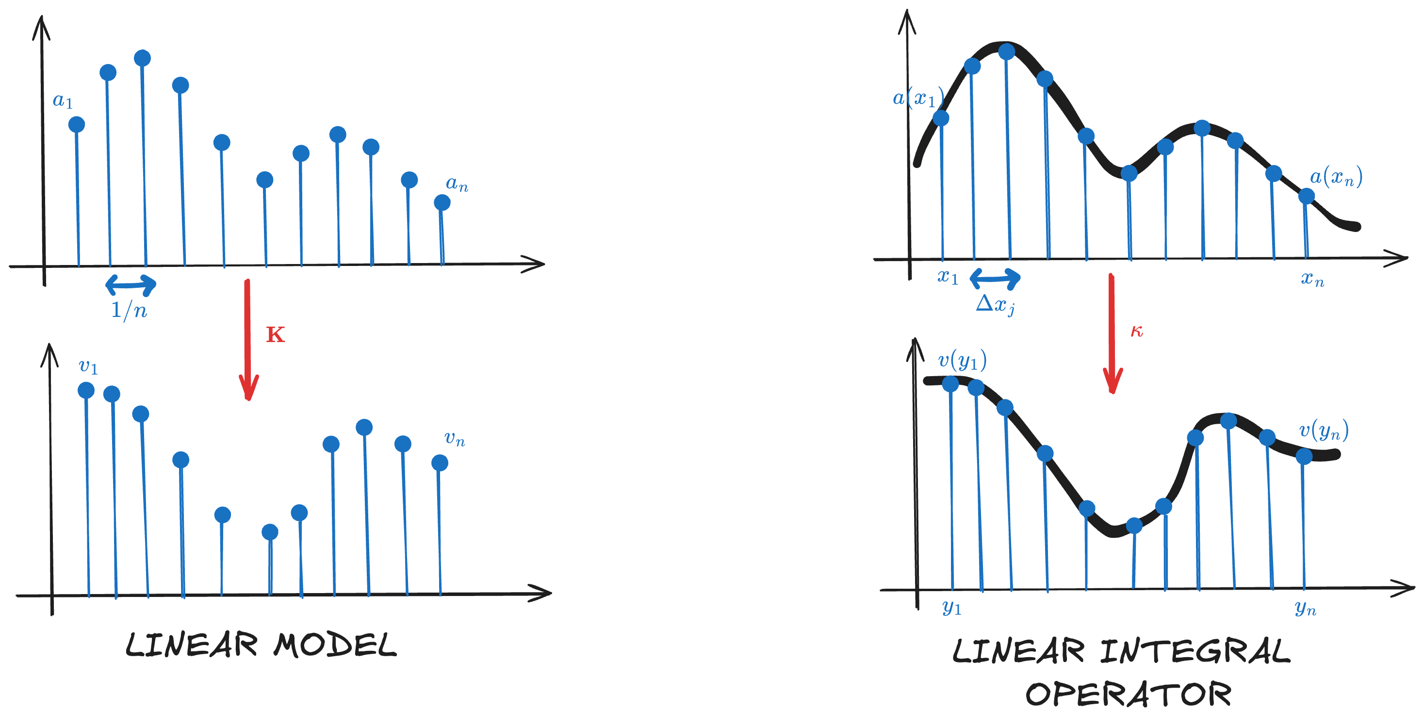Comparison of linear model and linear integral operator.

General Neural Operator Architecture

A neural operator architecture consists of multiple layers. First the input $a \in \mathcal{A}$ is transformed into a higher dimensional channel space representation $v_0(x) = P(a(x))$. Then we perform $T$ updates to obtain $v_T$. Finally, the output is obtained as $u(x) = Q(v_T(x))$.

The general transformation $v_t \mapsto v_{t+1}$ is defined as

\[\begin{equation} \label{eq:res-def} v_{t+1}(x) := \sigma \left( Wv_t(x) + \int \kappa_{\phi} (x, y) v_t(y)\text{d}y \right). \end{equation}\]

Compared to the definition in \eqref{eq:basic-def} here we have introduced the residual connection and the fact that $\kappa$ is parametrized by $\phi$.

Fourier Neural Operator

If we replace $\kappa_{\phi}(x, y)$ with $\kappa_{\phi}(x-y)$ in \eqref{eq:res-def} we obtain that the integral represents now a convolution.

Therefore, we can apply the convolutional theorem and obtain:

\[\begin{equation} \int \kappa_{\phi} (x - y) v_t(y)\text{d}y = \mathcal{F}^{-1}(\mathcal{F}(\kappa_{\phi}) \cdot \mathcal{F}(v_t))(x), \end{equation}\]

where $\mathcal{F}(\cdot)$ denotes the Fourier transform.

Next, we parametrize $\kappa_{\phi}$ directly in the Fourier domain by $R_{\phi}$.

The figure below highlights the steps of the Fourier Neural Operator (FNO) pipeline.

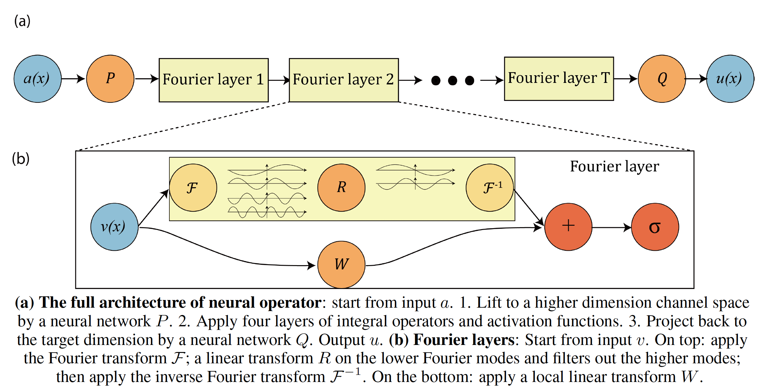Extracted from (Li et al., 2021).

Practical considerations

In general $v_t \in \mathbb{R}^{n \times d_v}$, where $d_v$ is the channel dimension, and $n$ is the number of points that we have used to discretize the domain.

In the Fourier domain we would also have that $\mathcal{F}(v_t) \in \mathbb{C}^{n \times d_v}$, meaning that we have a Fourier transform for each mode.

This would mean that we should learn a matrix $R_{\phi}$ for each mode. However, instead of using all the modes, only the first $k_{\text{max}}$ low frequency modes are used. Therefore, $R_{\phi} \in \mathbb{C}^{k_{\text{max}} \times d_v \times d_v}$ (for each of the $k_{\text{max}}$ modes, there’s a $ d_v \times d_v $ matrix that mixes the $d_v$ channels). Consequently, we also truncate the Fourier transform of the input signal $\mathcal{F}(v_t) \in \mathbb{C}^{k_{\text{max}} \times d_v}$.

The code below shows how this procedure works in practice.

import torch
import torch.nn as nn

batch, d_v, H, W = 8, 4, 64, 64  # example sizes
v_t = torch.randn(batch, d_v, H, W)

# FFT2: Convert to Fourier domain (complex tensor)
v_hat = torch.fft.rfft2(v_t, norm="ortho")  # shape: (batch, d_v, H, W//2 + 1)

k_max = 16
# Only apply weights to modes (kx, ky) where kx, ky <= k_max
# Create R as a complex tensor of shape (k_max, k_max, d_v, d_v)
R_real = nn.Parameter(torch.randn(k_max, k_max, d_v, d_v))
R_imag = nn.Parameter(torch.randn(k_max, k_max, d_v, d_v))
R = R_real + 1j * R_imag  # complex weights per mode


v_hat_out = torch.zeros_like(v_hat)  # same shape as input FFT

for i in range(min(k_max, v_hat.shape[2])):        # H direction (kx)
    for j in range(min(k_max, v_hat.shape[3])):    # W direction (ky)
        v_k = v_hat[:, :, i, j]  # shape: (batch, d_v) --- each frequency vector

        # Apply R(i,j): shape (d_v, d_v)
        R_ij = R[i, j]  # shape (d_v, d_v), complex

        # Batch matrix multiplication: (batch, d_v)
        v_hat_out[:, :, i, j] = torch.einsum("bd,dc->bc", v_k, R_ij)

v_out = torch.fft.irfft2(v_hat_out, s=(H, W), norm="ortho")  # shape: (batch, d_v, H, W)

Experiments

Here we show the results of training the FNO on the Darcy flow dataset with $16\times 16$ resolution and testing it on both $16\times 16$ and $32\times 32$ resolution. For the implementation we have used the Neural Operator library (Kossaifi et al., 2024; Kovachki et al., 2021).

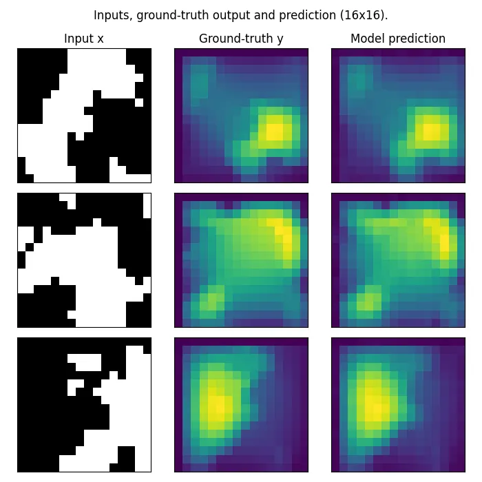Train and test on $16 \times 16$ resolution.

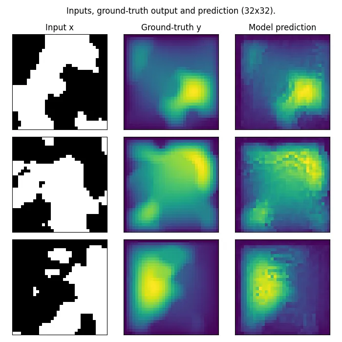Train on $16 \times 16$ resolution and test on $32 \times 32$ resolution.

References

1. Li, Z., Kovachki, N. B., Azizzadenesheli, K., liu, B., Bhattacharya, K., Stuart, A., & Anandkumar, A. (2021). Fourier Neural Operator for Parametric Partial Differential Equations. International Conference on Learning Representations.
2. Kossaifi, J., Kovachki, N., Li, Z., Pitt, D., Liu-Schiaffini, M., George, R. J., Bonev, B., Azizzadenesheli, K., Berner, J., & Anandkumar, A. (2024). A Library for Learning Neural Operators.
3. Kovachki, N. B., Li, Z., Liu, B., Azizzadenesheli, K., Bhattacharya, K., Stuart, A. M., & Anandkumar, A. (2021). Neural Operator: Learning Maps Between Function Spaces. CoRR, abs/2108.08481.