
Transformers revolutionized sequence modeling with their attention-based, non-recurrent architecture. This tutorial builds up the transformer model step by step—from self-attention and positional encoding to encoder-decoder attention and multi-head mechanisms—explaining each concept with math, visuals, and practical insights. Ideal for readers seeking a solid, intuitive grasp of how transformers really work under the hood.
Transformers have been proposed in the paper “Attention is all you need” by Ashish Vaswani et al. (Vaswani et al., 2017). Transformers are intrinsically related to Large Language Models (LLMs), as LLMs are built upon the transformer architecture.
But what exactly are transformers?
Essentially, transformers are neural networks designed for sequential data or time series. What distinguishes them from other neural networks designed for the same purposes are the facts that transformers are non-recurrent models and use the attention mechanism.
Because of these two main characteristics they offer several advantages compared to LSTM:
- Handle long-range dependencies thanks to the self-attention mechanism
- Faster than LSTM because they can process the input sequence in parallel
- Easier to train thanks to the absence of recurrent connections, they do not suffer from exploding or vanishing gradient issues
- Generate more meaningful representations that better capture the relationships between words and their contexts compared to the LSTM’s fixed-size hidden state (in natural language processing)
In this tutorial, I’m going to walk you through understanding the transformer model. Given its complexity, I’ll start with the basics and gradually dive into more intricate details of the model step by step.
The Model
When having a first glimpse of the model, we see that it consists of a stack of encoders and decoders. Additionally, we see that each encoder contain a self-attention block, whereas the decoder has both a (masked) self-attention block and a so called encoder-decoder attention block.
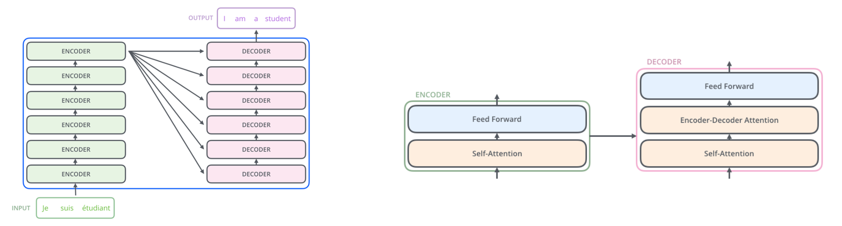 Figure 1: First glimpse of the model.
By taking a closer look at the transformer encoder in Figure 2 we notice that the words (represented as embeddings) flow in parallel. Additionally, we can see that the embeddings are handled independently except for the self-attention block, which creates dependencies between the different embeddings. Also, so far, the position of the different words does not matter.
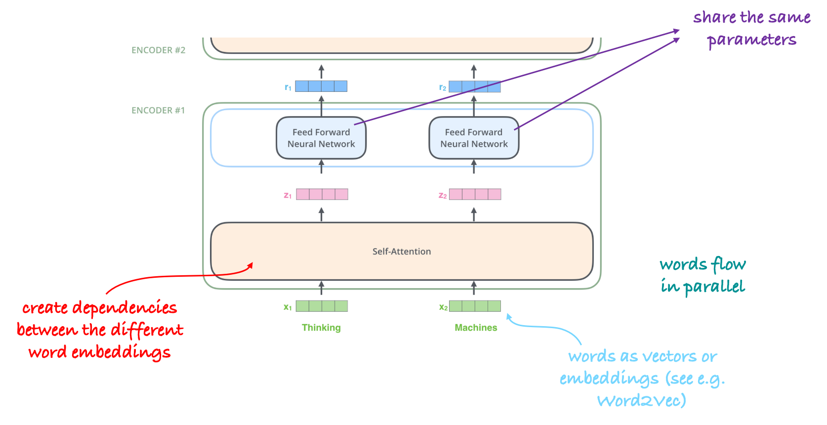 Figure 2: Transformer encoder.
Self-attention
For each embedding we compute query, key and value, by multiplying with the trainable parameters $\vW_q$, $\vW_k$, and $\vW_v$, respectively. As illustrated in Figure 3 we can see that the parameters are shared between the different embeddings.
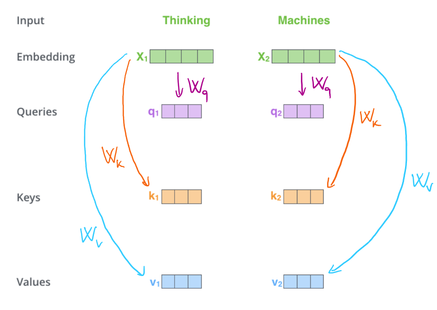 Figure 3: Computing queries, keys, and values.
Afterward, we proceed to compute self-attention. As depicted in Figure 4, for each embedding, we calculate attention scores by multiplying the corresponding query with the keys. These scores are then transformed into attention weights through a softmax operation.
Then the new embeddings are obtained as a weighted sum of the values. 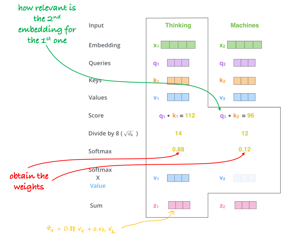 Figure 4: Self-attention.
But how does attention mechanism enhance the embeddings?
Attention enhances embeddings in neural networks by introducing a context-aware weighting system that leverages other embeddings to improve the encoding of the current embedding. For instance, upon examining the changes from $\vx_1$ to $\vz_1$, it becomes evident that $\vz_1$ now integrates additional information derived from the other embeddings.
In essence, attention allows the transformer to dynamically emphasize relevant embeddings while downplaying less relevant ones, thereby refining the representation of each embedding based on the context provided by others. This capability significantly boosts the network’s ability to capture intricate relationships and dependencies within data, making it particularly powerful in tasks requiring nuanced understanding and context-aware processing.
In this example, we can see that the embedding corresponding to the pronoun “it” focuses most on the embedding corresponding to the word “animal”.
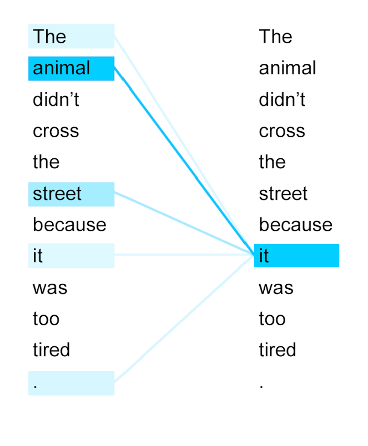 Figure 5: Self-attention example.
Positional encoding
The model presented so far is permutation invariant, in the sense that a permutation of the input embeddings (shuffling of the words of the input sentence) corresponds to an equivalent permutation of the embeddings at the encoder outputs, and does not change the content of each embedding.
Therefore, we need a way to account for the order of the words in the input sequence. In LSTM this is done automatically because of the recurrent/sequential nature of the model itself (inputs are fed one by one following their order of appearance).
To account for the order of the words we add a vector with a specific pattern to each input embedding, see Figure 6.
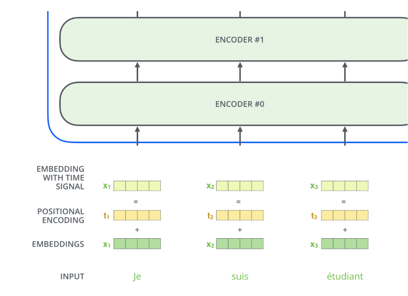 Figure 6: Positional encoding overview.
The positional encoding for each embedding is obtained using the formula below:
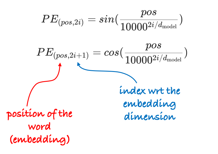
where the index $i$ varies from $0$ up to $\frac{d_{\text{model}}}{2} - 1$. In particular, we can observe that when $i \ge 1$ the denominator is larger than $1$ and the frequency of the sinusoids decreases.
Let’s visualize this with an example. In this example we assume that $d_{\text{model}} = 50$, and we observe what happens to the values of $pos \in \{0, 1, 2, 3\}$.
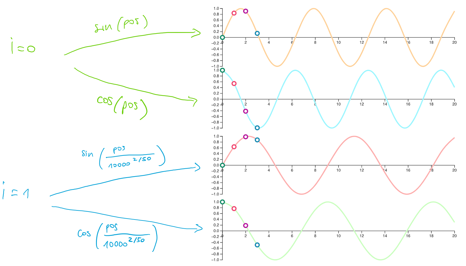 Figure 7: Positional encoding example.
If we then construct a matrix that has the $pos$ index on the y-axis and the $i$ index on the x-axis we can observe the pattern in Figure 8.
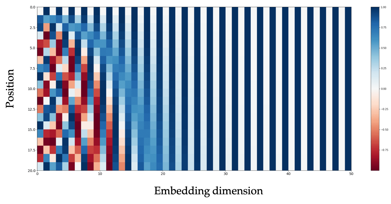 Figure 8: Positional encoding pattern.
In particular, we can observe that the values of the first 20 positions for higher indices of the embedding dimension remain nearly constant.
What this mean?
To have an intuition we can think about binary numbers. In Figure 8, we can see that numbers closer to each other share more of the most significant digits. Similarly, with positional encoding, position indices that are close to each other share the values of most of the indices of the embedding dimension.
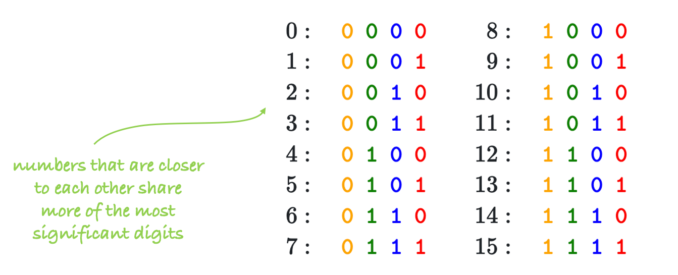 Figure 8: Positional encoding intuition.
Another motivation for positional encoding is given in the paper: “We chose this function because we hypothesized it would allow the model to easily learn to attend by relative positions, since for any fixed offset $k$, $PE_{pos+k}$ can be represented as a linear function of $PE_{pos}$.”
In essence, what the authors are saying is that we can always find a $2 \times 2$ matrix $\vM$ that only depends on $k$ such that
where $\omega_i = \frac{1}{10000^{2i/d_{\text{model}}}}$.
Transformer decoder
The transformer decoder uses both a masked self-attention and an encoder-decoder attention.
Why masking?
In the decoder, the self-attention layer is only allowed to attend to earlier positions in the output sequence. This means we can’t predict words based on future words. Masking future positions (setting them to -inf) before the softmax step in the self-attention calculation ensures this restriction is enforced.
In Pytorch we would simply do
1

    attn_weights = F.softmax(scores + mask, dim=-1)
This procedure is very important because it allows us to train the decoder in parallel. However, during the operational time, the inference in the decoder is done sequentially until the embedding of “end of sentence” is reached.
The Encoder-Decoder Attention layer, instead, works like the self-attention, except it creates its Queries matrix from the layer below it, and takes the Keys and Values matrix from the output of the encoder.
Transformer in action
In Figure 9 we see how the transformer predicts the sentence word by word1. In the final layer of the decoder the softmax is used to take the word with the highest probability.
 Figure 9: Transformer in action.
Is this the whole story? ![]()
Indeed, the model has some more details…
More details
If we take a closer look at the encoder block2 we see that it contains also residual connections and layer normalization.
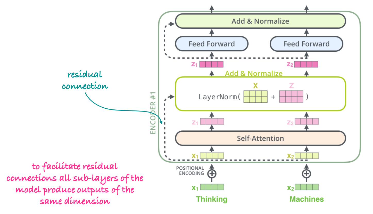 Figure 10: Additional components.
The main purpose of using residual connections in transformers is to address the vanishing gradient problem. During the backpropagation process, gradients can become extremely small as they are propagated backward through many layers. As a result, the weights in the early layers of the network may not get updated effectively, leading to slow or stalled learning and difficulty in training very deep networks. The residual connections also preserve the positional encoding information which is added only at the beginning of the model.
Why LayerNorm instead of BatchNorm?
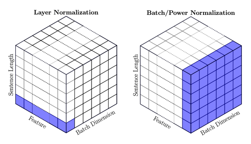 Figure 11: LayerNorm vs. BatchNorm.
In Figure 11 we see the differences between LayerNorm and BatchNorm. In essence LayerNorm is preferred for the following reasons:
- Input sequences can have varying lengths. BatchNorm, which relies on batch statistics, is not suitable
- Order of the words in a sentence matters
- During decoding, we process one embedding at a time
- More time-efficient
Multi-head attention
Once we understand the concept of self-attention, the idea of multi-head attention becomes almost straightforward.
The motivation for multi-head attention is explained in the paper: “Instead of performing a single attention, we found it beneficial to linearly project the queries, keys and values $h$ times with different, learned linear projections.”
Furthermore, the paper states: On each of these projected versions of queries, keys and values we then perform the attention function in parallel. The output values are concatenated and once again projected, resulting in the final values. This procedure is illustrated in Figure 12.
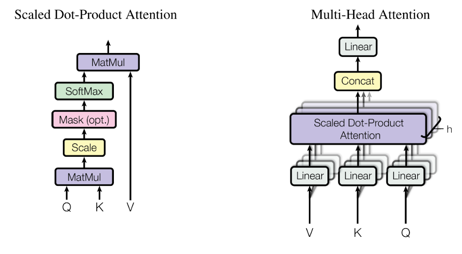 Figure 12: Multi-head attention.
And that wraps up my post!
Thank you for your attention! ![]()
If you enjoyed it, spread the love with a ![]() or share your thoughts below!
or share your thoughts below!
References
- Vaswani, A., Shazeer, N., Parmar, N., Uszkoreit, J., Jones, L., Gomez, A. N., Kaiser, Ł., & Polosukhin, I. (2017). Attention is All you Need. Advances in Neural Information Processing Systems, 30.
The figures, onto which I’ve added my notes, have been extracted from: