
I’ve recently attended the Machine Learning Summer School in Kraków (Poland), where I particularly enjoyed Yarin Gal’s talk on uncertainty in deep learning. In this post, I will summarize the main ideas from his presentation.
Why is uncertainty important?
Suppose we have trained a model that, given an image of a dog as input, outputs the breed of that particular dog. If we provide this model with an image of a cat, it would still output a dog breed. However, what we actually want is for the model to tell us what it knows and what it does not know. And this is where uncertainty comes into play. Notably, model uncertainty information becomes crucial in systems that make decisions affecting human life.
Bayesian Neural Networks
To formalize the problem mathematically, let’s assume we are given training inputs $X \coloneqqf \{ \vx_1, \dots, \vx_N\}$ and their corresponding outputs $Y \coloneqqf \{ \vy_1, \dots, \vy_N\}$. In regression, we would like to find the parameters $\param$ of a function $f_{\param}$ such that $\vy = f_{\param}(\vx)$.
In the Bayesian framework, we start by specifying a prior distribution over the parameter space, $p(\param)$. This distribution reflects our initial beliefs about which parameters are probable candidates for generating our data, before any data points are observed. As we observe data, this prior distribution is updated to form a posterior distribution, which encapsulates the relative likelihoods of different parameter values given the observed data. To complete this Bayesian inference process, we also define a likelihood distribution, $p(\vy \mid \vx, \param)$, which specifies the probability of observing the data $\vy$ given the parameters $\param$ and the input $\vx$.
Given our dataset we then look for the posterior distribution $p(\param \mid X, Y)$ using the Bayes’ theorem:
In Bayesian inference, a critical component is the normalizer, also referred to as model evidence:
However, this marginalization cannot be done analytically.
Variational inference
As the true posterior $p(\param \mid X, Y)$ is hard to compute we define a variational distribution $q_{\bphi}(\param)$, parameterized by $\bphi$ which is simple to evaluate. We would like our approximating distribution to be as close as possible to the true posterior. Therefore, in other words we want to minimize the KL divergence between the two distributions:
It can be shown that minimizing this divergence is equivalent to maximizing the evidence lower bound (ELBO) expression:
Monte-Carlo Dropout
Interestingly this objective is identical to the objective of a dropout neural network (with some regularization terms included).
What does this mean?
This implies that the optimal weights obtained by optimizing a neural network with dropout are equivalent to the optimal variational parameters in a Bayesian neural network with the same architecture. Consequently, a network trained using dropout inherently functions as a Bayesian neural network, thereby inheriting all the properties associated with Bayesian neural networks.
Essentially, this means that we can model uncertainty using dropout at test time! We refer to this procedure as Monte-Carlo dropout. For example, we can estimate the first two moments of the predictive distribution empirically by running:
1
2
3
4
5

y = []
for _ in range(10):
    y.append(model.output(x, dropout=True))
y_mean = numpy.mean(y)
y_var = numpy.var(y)
In Figure 1 we see an example of Monte-Carlo dropout applied to the case of $\text{CO}_2$ concentration prediction.
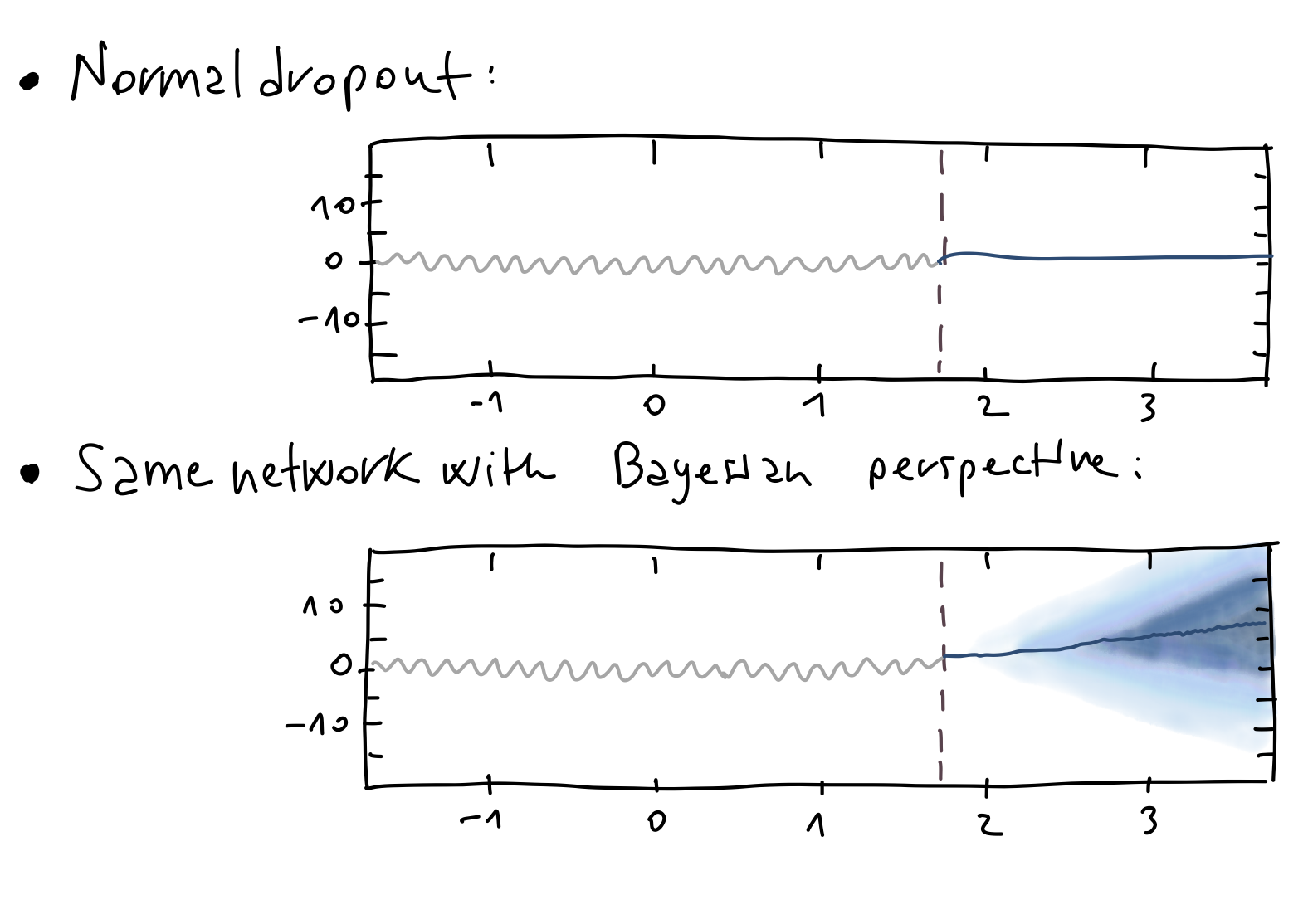 Figure 1: $\text{CO}_2$ concentration prediction.
To summarize, in regression, we quantified predictive uncertainty by examining the sample variance across multiple stochastic forward passes.
Uncertainty in classification
For uncertainty in classification we can consider different measures that capture different notions of uncertainty. One possible approach is to look at the predictive entropy. This quantity represents the average amount of information within the predictive distribution:
where the summation is over all possible classes $c$ that $y$ can assume. For a given test point $\vx$, the predictive entropy reaches its highest value when all classes are predicted with equal probability (indicating complete uncertainty). Conversely, it reaches its lowest value of zero when one class is predicted with a probability of 1 and all other classes with a probability of 0 (indicating complete certainty in the prediction).
In particular, the predictive entropy can be estimated by gathering the probability vectors from $T$ stochastic forward passes through the network. For each class $c$, we average the probabilities from each of the $T$ probability vectors.
In formulas, we replace $p(y = c \mid \vx, \mathcal{D}_{\text{train}})$ with $\frac{1}{T} \sum_t p(y = c \mid \vx, \hat{\param}_t)$, where ${\hat{\param}_{t}} \sim {q_{\bphi}} (\param)$.
A better alternative to the predictive entropy is the mutual information between the prediction $y$ and the posterior over the model parameters $\param$:
The expression can be then approximated as
where the term in magenta denotes the entropy, and the term in orange denotes the negative average of the entropies.
Example
To better understand why the mutual information better capture the model uncertainty let’s consider the following binary classification problem.
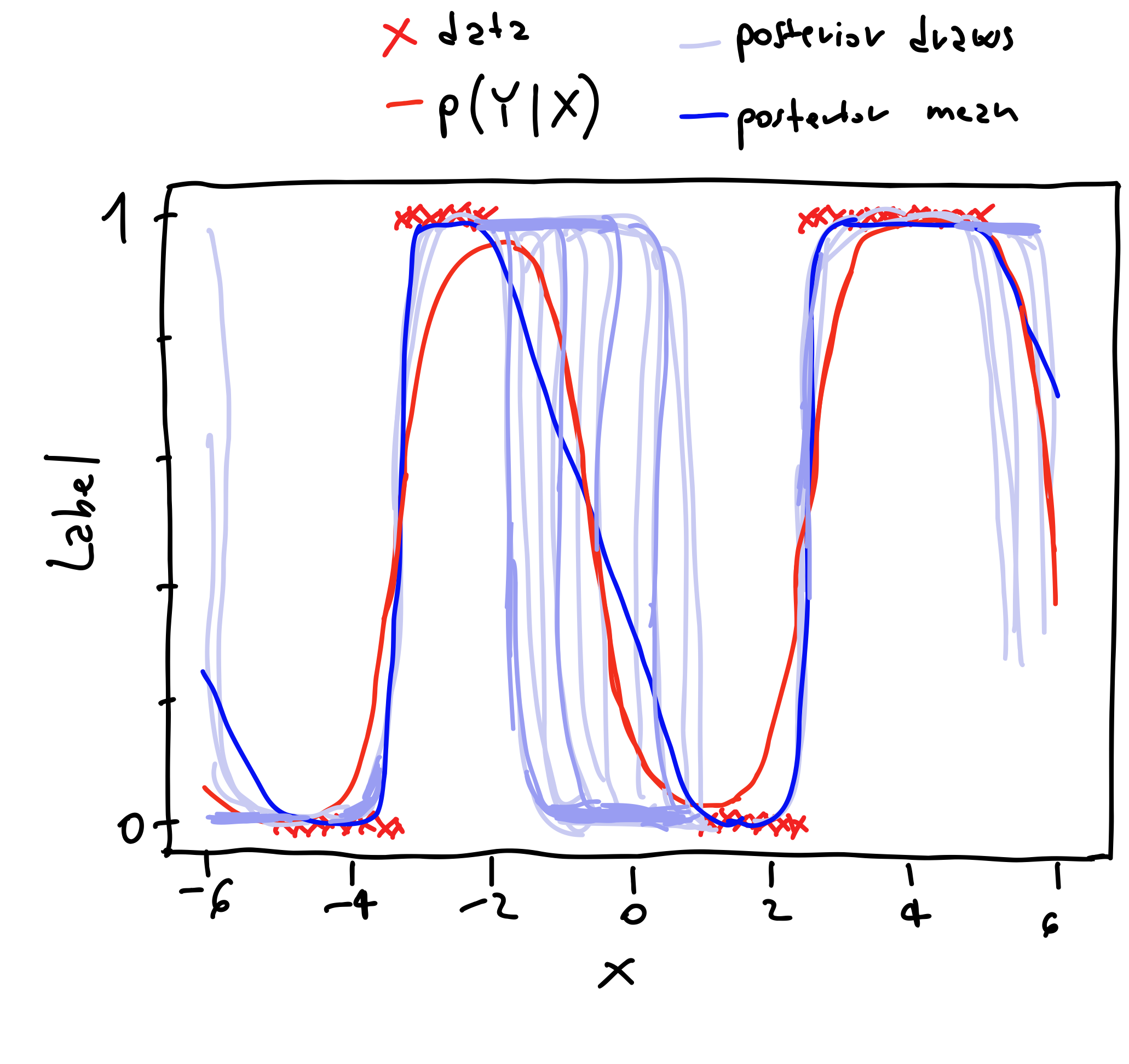 Figure 2: Binary classification example.
Here we have a scalar $x$ that can assume continuous values between $(-6, 6)$, and the corresponding labels $\{0, 1\}$. In the figure we also highlight the posterior draws, and the posterior mean obtained by averaging the posterior draws.
Now let’s see what happens when we compute both the entropy and the mutual information using the expressions above.
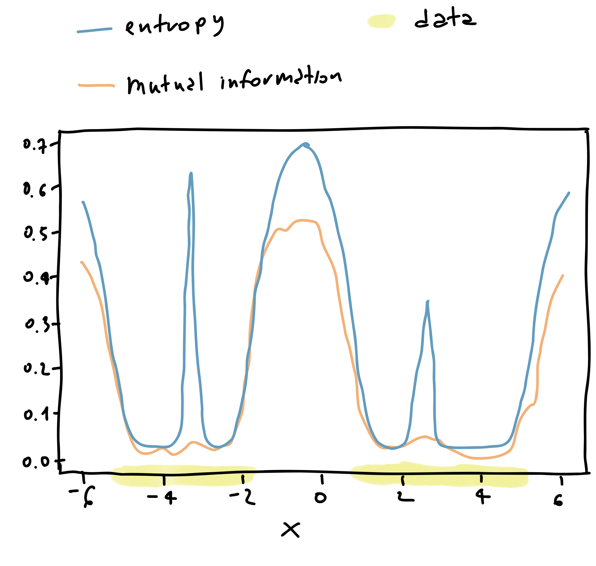 Figure 3: Uncertainty in classification.
In particular, for values of $x \approx -3$ we see that the predictive entropy, that is the entropy of the thick blue line in Figure 3 is quite high. The same happens in the surroundings of $x \approx 0$ and $x \approx 3$. On the other hand, the mutual information is quite low for $x \approx -3$ and $x \approx 3$, whereas it is still high for $x\approx 0$.
Why is this the case?
To understand this behavior, we can notice that in the interval $(-2, 1)$, where we have no data, the lines corresponding to the posterior draws mostly belong to two categories. The categories are illustrated in Figure 4.
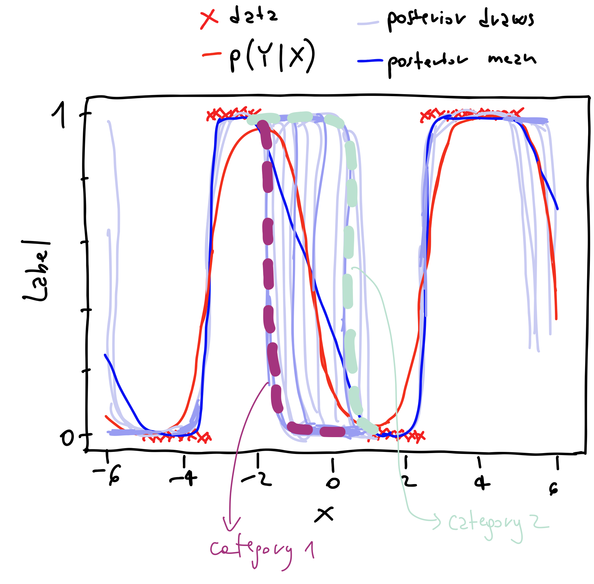 Figure 4: Understanding mutual information results.
Basically, most of the posterior draws indicate that the prediction in that interval should either be $0$ or $1$. Consequently, when evaluating the mutual information, the term in orange in formula \eqref{eq:mutual-info} is essentially an average of $0$. Therefore, the mutual information in that interval is high because we subtract a small number from a large number.
On the other hand, for values of $x \approx -3$ or $x \approx 3$, the posterior draws overlap with the thick blue line, meaning that the average of the entropies is essentially equal to the entropy. Therefore, the mutual information is low.
What is then the point?
The point is that thanks to the mutual information metric we can better capture the model’s uncertainty which is due to lack of data.
Active learning
The described approaches of predictive entropy and mutual information becomes very useful in the context of active learning. The active learning setup can be summarized by the following steps:
- train a model with labeled samples
- extract data from the pool of unlabeled data
- ask the expert to label the chosen data
- retrain the model
How to choose the data from the unlabeled pool?
Well, we take those that maximize the mutual information! ![]()